EKF SLAM on a TurtleBot3

Overview

Built a full SLAM stack from the ground up for a TurtleBot3 differential-drive robot in ROS 2. The robot uses a LIDAR to detect cylindrical landmarks and maintains a joint estimate of its own pose and all landmark positions.

The stack was cross-compiled for the TurtleBot3’s ARM processor (aarch64) and deployed live on the robot.

Packages

Package	Role
turtlelib	2D rigid-body transforms and differential-drive kinematics
nusim	ROS 2 simulator and visualizer for TurtleBot3
nuturtle_description	URDF and robot description files
nuturtle_interfaces	Custom ROS 2 service definitions
nuturtle_control	Odometry, low-level control
nuslam	EKF SLAM with unknown data association

Odometry

Wheel encoder readings are integrated via the differential-drive kinematic model in turtlelib to estimate the robot’s pose. Odometry accumulates drift over time, which the SLAM filter is designed to correct.

EKF SLAM

The Extended Kalman Filter tracks a joint state vector $\mathbf{x}$ containing both the robot pose and all landmark positions:

$$\mathbf{x} = \begin{bmatrix} x & y & \theta & m_{x_1} & m_{y_1} & \cdots & m_{x_n} & m_{y_n} \end{bmatrix}^T$$

Each timestep has two steps:

Predict — motion model

A control input $\mathbf{u} = (v, \omega)$ (linear and angular velocity from wheel encoders) propagates the robot pose forward via the differential-drive kinematic model. The covariance is inflated by process noise $Q$:

$$\hat{\mathbf{x}}_k = f(\mathbf{x}_{k-1}, \mathbf{u}_k)$$ $$\hat{\Sigma}_k = A_k \Sigma_{k-1} A_k^T + Q$$

where $A$ is the Jacobian of the motion model with respect to the state.

Update — measurement model

The LIDAR produces a point cloud that is processed through a perception pipeline — clustering, circle regression, and classification — to detect cylindrical landmarks and publish their relative positions on the map. These detections are what feed the measurement model. The Kalman gain $K$ then weights how much to trust the sensor versus the prediction:

$$K = \hat{\Sigma}_k H_k^T (H_k \hat{\Sigma}_k H_k^T + R)^{-1}$$ $$\mathbf{x}_k = \hat{\mathbf{x}}_k + K(\mathbf{z}_k - h(\hat{\mathbf{x}}_k))$$ $$\Sigma_k = (I - KH_k)\hat{\Sigma}_k$$

where $H$ is the Jacobian of the measurement function $h$.

SLAM in simulation

The nuslam package runs an EKF that maintains a joint state of the robot pose $(x, y, \theta)$ and all detected landmark positions $(m_{x_i}, m_{y_i})$. The filter supports two modes:

• Known data association — landmark IDs are provided directly by the simulator.
• Unknown data association — landmarks are matched to the existing map, with a distance threshold to initialize new landmarks.

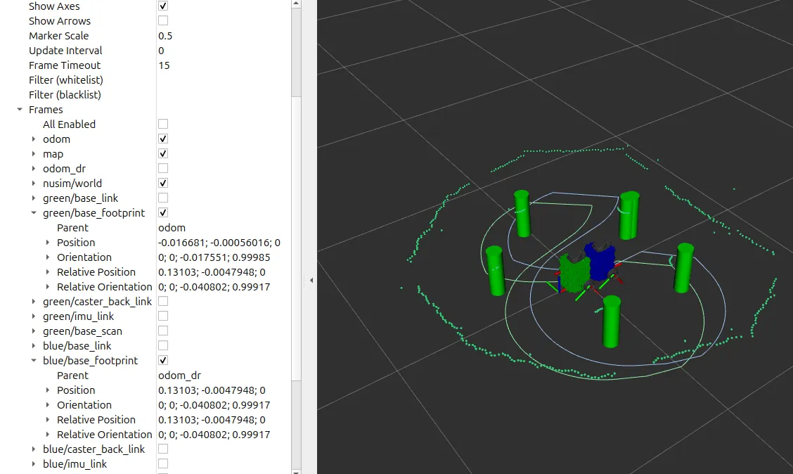
RViz displays the ground-truth robot, the SLAM estimate, the odometry estimate, and the estimated and actual landmark positions simultaneously.

SLAM in the real world

The filter was deployed on a physical TurtleBot3 navigating an environment of cylindrical landmarks. After a full loop, the SLAM estimate returned close to the origin while odometry had drifted significantly:

Estimator	x (m)	y (m)	θ (rad)
SLAM	−0.016	−0.001	−0.018
Odometry	0.131	−0.005	−0.040